Predictions

This is a guide on utilizing the PreFab Python API to anticipate the fabrication outcomes of nanoscale structures, specifically a 200 nm-wide cross structure on a silicon-on-insulator (SOI) e-beam process. This guide is structured as follows:

1. Preparing a device image for prediction
2. Executing a prediction
3. Analyzing a prediction

Required libraries

To begin, we need to import the necessary libraries:

import matplotlib.pyplot as plt
import prefab as pf

Loading a device image

The first step involves preparing a device image for prediction. Refer to GDS for a guide on reading from GDS layout files. This requires loading an image of a device as a numpy matrix with binary pixel values: 0 or 1. In this tutorial, we'll use an image of a cross, but feel free to explore with other structures available in /devices or on GitHub, or include your own images.

The image scale should ideally be 1 nm/px. If not, ensure you specify the actual length of the device image (in nanometers) when loading the image. In this case the image is 256 px wide, and the device is 256 nm wide, so we can omit the img_length_nm parameter.

IMG_LENGTH_NM = 256
device = pf.load_device_img(
    path="../devices/target_32x128_256x256.png",
    img_length_nm=IMG_LENGTH_NM
)

plt.imshow(device)
plt.title("Nominal Device")
plt.ylabel("Distance (nm)")
plt.xlabel("Distance (nm)")
plt.show()

Making a prediction

In the next step, we proceed with the prediction. Each model is labeled by its fabrication facility and process name, model version, and dataset version. Refer to Models for the list of available models.

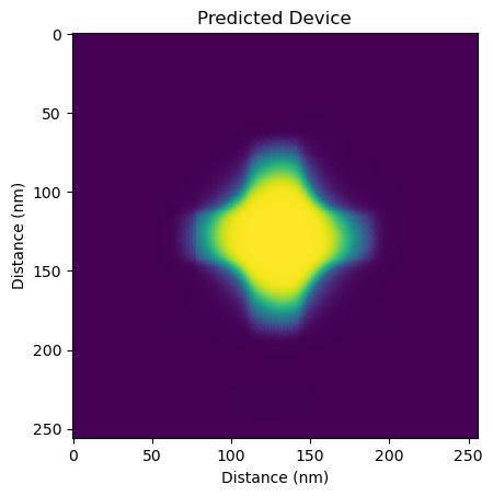
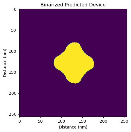
With prediction, a binarized output can be chosen. The predictor, by default, produces raw predictions, which includes "fuzzy" areas of the structure that might vary between different fabrication runs or even different device instances on the same chip. When binarized, the predictor outputs the most probable fabrication outcome. Post-prediction binarization is also an option, as shown below.

# Note: Initial prediction may take longer due to server startup and model loading.
#       Subsequent predictions will be quicker.

MODEL_NAME = "ANT_NanoSOI"
MODEL_TAGS = "v5-d4"
prediction = pf.predict(
  device=device,
  model_name=MODEL_NAME,
  model_tags=MODEL_TAGS,
  binarize=False
)

plt.imshow(prediction)
plt.title("Predicted Device")
plt.ylabel("Distance (nm)")
plt.xlabel("Distance (nm)")
plt.show()

plt.imshow(pf.binarize(prediction))
plt.title("Binarized Predicted Device")
plt.ylabel("Distance (nm)")
plt.xlabel("Distance (nm)")
plt.show()

Prediction analysis

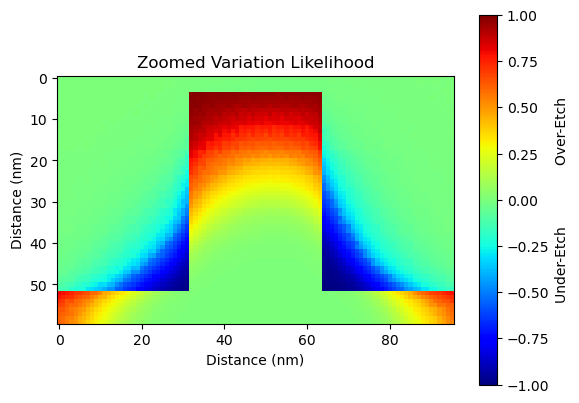
In the fabrication process, each run will have slight variations due to a multitude of factors such as equipment precision, environmental conditions, and material inconsistencies. These variations can lead to differences in the final fabricated device compared to the original design.

The prediction analysis technique mentioned in the document helps to identify areas of high uncertainty in the fabrication process. By plotting the variations between the nominal (or intended) device and the predicted outcome, we can visualize these areas of uncertainty. For example, potential rounding of the cross' corners is identified as an area of high uncertainty. This means that in each fabrication run, the exact shape of the corners might vary, but they will generally tend to round off.

This analysis does not provide a deterministic prediction of the fabrication outcome, but rather a probabilistic one. It gives us a 'region of uncertainty' within which the actual fabrication outcome is likely to fall. Understanding this region of uncertainty is crucial for design refinement and process optimization. It allows designers to anticipate potential fabrication variations and adjust their designs accordingly to achieve the desired performance.

variation = device - prediction
plt.imshow(variation, cmap="jet", vmin=-1, vmax=1)
plt.title("Variation Likelihood")
plt.ylabel("Distance (nm)")
plt.xlabel("Distance (nm)")
cb = plt.colorbar()
cb.set_label("Under-Etch              Over-Etch")
plt.show()

plt.imshow(variation[60:120, 80:-80], cmap="jet", vmin=-1, vmax=1)
plt.title("Zoomed Variation Likelihood")
plt.ylabel("Distance (nm)")
plt.xlabel("Distance (nm)")
cb = plt.colorbar()
cb.set_label("Under-Etch Over-Etch")
plt.show()