GDS

This is a guide on using the PreFab Python API to predict the fabrication outcomes of a nanobeam structure, specifically imported from a GDS file, on a silicon-on-insulator (SOI) e-beam process. The tutorial encompasses:

1. Importing a device from a GDS layout cell
2. Executing a prediction
3. Analyzing a prediction
4. Writing a predicted device back to a GDS file

Required libraries

To begin, we need to import the necessary libraries:

python import matplotlib.pyplot as plt
import prefab as pf import gdstk

Loading a GDS cell

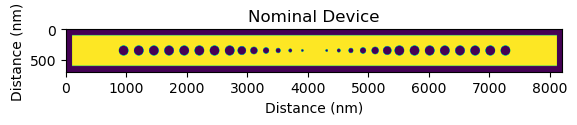
We commence by importing a nanobeam device from a GDS file, transforming the geometric data into a numpy matrix with pixel values of either 0 or 1. We use a specific nanobeam design in this tutorial, but feel free to explore with other structures available in /devices/devices.gds or on GitHub, or include your own layouts.

device = pf.load_device_gds(path="../devices/devices.gds", cell_name="nanobeam")

plt.imshow(device)
plt.title("Nominal Device")
plt.ylabel("Distance (nm)")
plt.xlabel("Distance (nm)")
plt.show()

Making a prediction

In the next step, we proceed with the prediction. Each model is labeled by its fabrication facility and process name, model version, and dataset version. Refer to Models for the list of available models.

With prediction, a binarized output can be chosen. The predictor, by default, produces raw predictions, which includes "fuzzy" areas of the structure that might vary between different fabrication runs or even different device instances on the same chip. When binarized, the predictor outputs the most probable fabrication outcome. Post-prediction binarization is also an option, as shown below.

# Note: Initial prediction may take longer due to server startup and model loading.
#       Subsequent predictions will be quicker.

MODEL_NAME = "ANT_NanoSOI"
MODEL_TAGS = "v5-d4"
prediction = pf.predict(
  device=device,
  model_name=MODEL_NAME,
  model_tags=MODEL_TAGS,
  binarize=False
)

plt.imshow(prediction)
plt.title("Predicted Device")
plt.ylabel("Distance (nm)")
plt.xlabel("Distance (nm)")
plt.show()

Prediction analysis

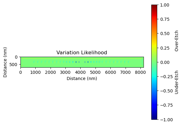
In the fabrication process, each run will have slight variations due to a multitude of factors such as equipment precision, environmental conditions, and material inconsistencies. These variations can lead to differences in the final fabricated device compared to the original design.

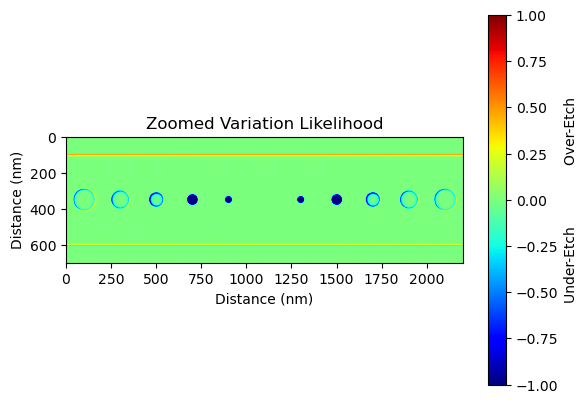
The prediction analysis technique mentioned in the document helps to identify areas of high uncertainty in the fabrication process. By plotting the variations between the nominal (or intended) device and the predicted outcome, we can visualize these areas of uncertainty. For our nanobeam, for instance, we may notice filling of the first two innermost holes and a general dilation of the larger holes. These are fabrication process artifacts, and understanding their potential appearance helps us to better predict and plan for the actual outcome.

This analysis does not provide a deterministic prediction of the fabrication outcome, but rather a probabilistic one. It gives us a 'region of uncertainty' within which the actual fabrication outcome is likely to fall. Understanding this region of uncertainty is crucial for design refinement and process optimization. It allows designers to anticipate potential fabrication variations and adjust their designs accordingly to achieve the desired performance.

variation = device - prediction
plt.imshow(variation, cmap="jet", vmin=-1, vmax=1)
plt.title("Variation Likelihood")
plt.ylabel("Distance (nm)")
plt.xlabel("Distance (nm)")
cb = plt.colorbar()
cb.set_label("Under-Etch              Over-Etch")
plt.show()

plt.imshow(variation[0:-1, 3000:-3000], cmap="jet", vmin=-1, vmax=1)
plt.title("Zoomed Variation Likelihood")
plt.ylabel("Distance (nm)")
plt.xlabel("Distance (nm)")
cb = plt.colorbar()
cb.set_label("Under-Etch Over-Etch")
plt.show()

Writing the predicted device to a GDS file

Lastly, we generate a GDS cell for the predicted binarized device and add it back to the original GDS library using the gdstk package. The GDS file with the original and predicted devices can then be exported for further use or analysis.

gds_library = gdstk.read_gds("../devices/devices.gds")
predicted_nanobeam_cell = pf.device_to_cell(
  device=pf.binarize(prediction),
  cell_name="nanobeam_p",
  library=gds_library,
  resolution=1,
  layer=(9, 0),
)
origin = (-device.shape[1] / 2 / 1000, -device.shape[0] / 2 / 1000)
gds_library["nanobeam"].add(
  gdstk.Reference(cell=predicted_nanobeam_cell, origin=origin)
)
gds_library.write_gds(outfile="../devices/devices.gds")